11 Day 11 (June 15)
11.1 Announcements
Assignment 3 is posted and due Friday
Vote on if tomorrow should be a work day?
Recommended reading
- Chapters 3 and 4 (pgs 33 - 58) in Linear Models with R
Questions and comments from journal
- “I am still trying to understand how we know if the estimated slopes from a linear model are reliable.”
- “It seems like results from models can then lead to more questions. Are those questions then incorporated into the model to account for that new question or does it lead to needing a new model entirely?”
- Comment on questioning model-based estimates or conclusions (return to deer example).
11.2 Maximum Likelihood Estimation
- Maximum likelihood estimation for the linear model
- Assume that \(\mathbf{y}\sim \text{N}(\mathbf{X}\boldsymbol{\beta},\sigma^2\mathbf{I})\)
- Write out the likelihood function \[\mathcal{L}(\boldsymbol{\beta},\sigma^2)=\prod_{i=1}^n\frac{1}{\sqrt{2\pi\sigma^2}}\textit{e}^{-\frac{1}{2\sigma^2}(y_{i} - \mathbf{x}_{i}^{\prime}\boldsymbol{\beta})^2}.\]
- Maximize the likelihood function
- First take the natural log of \(\mathcal{L}(\boldsymbol{\beta},\sigma^2)\), which gives \[\mathcal{l}(\boldsymbol{\beta},\sigma^2)=-\frac{n}{2}\text{ log}(2\pi\sigma^2) - \frac{1}{2\sigma^2}\sum_{i=1}^{n}(y_{i} - \mathbf{x}_{i}^{\prime}\boldsymbol{\beta})^2.\]
- Recall that \(\sum_{i=1}^{n}(y_{i} - \mathbf{x}_{i}^{\prime}\boldsymbol{\beta})^2 = (\mathbf{y} - \mathbf{X}\boldsymbol{\beta})^{\prime}(\mathbf{y} - \mathbf{X}\boldsymbol{\beta})\)
- Maximize the log-likelihood function \[\underset{\boldsymbol{\beta}, \sigma^2}{\operatorname{argmax}} -\frac{n}{2}\text{ log}(2\pi\sigma^2) - \frac{1}{2\sigma^2}(\mathbf{y} - \mathbf{X}\boldsymbol{\beta})^{\prime}(\mathbf{y} - \mathbf{X}\boldsymbol{\beta})\]
- Visual for data \(\mathbf{y}=(0.16,2.82,2.24)'\) and \(\mathbf{x}=(1,2,3)'\)
- Three ways to do it in program R
- Using matrix calculus and algebra
# Data
y <- c(0.16,2.82,2.24)
X <- matrix(c(1,1,1,1,2,3),nrow=3,ncol=2,byrow=FALSE)
n <- length(y)

# Maximum likelihood estimation using closed from estimators
beta <- solve(t(X)%*%X)%*%t(X)%*%y
sigma2 <- (1/n)*t(y-X%*%beta)%*%(y-X%*%beta)

beta
## [,1] ## [1,] -0.34 ## [2,] 1.04## [,1] ## [1,] 0.5832- Using modern (circa 1970’s) optimization techniques
# Maximum likelihood estimation estimation using the Nelder-Mead algorithm
y <- c(0.16,2.82,2.24)
X <- matrix(c(1,1,1,1,2,3),nrow=3,ncol=2,byrow=FALSE)

negloglik <- function(par){
beta <- par[1:2]
sigma2 <- par[3]
-sum(dnorm(y,X%*%beta,sqrt(sigma2),log=TRUE))
}
optim(par=c(0,0,1),fn=negloglik,method = "Nelder-Mead")
## $par ## [1] -0.3397162 1.0398552 0.5831210 ## ## $value ## [1] 3.447978 ## ## $counts ## function gradient ## 150 NA ## ## $convergence ## [1] 0 ## ## $message ## NULL- Using modern and user friendly statistical computing software
# Maximum likelihood estimation using lm function
# Note: estimate of sigma2 is not the MLE!
df <- data.frame(y = c(0.16,2.82,2.24),x = c(1,2,3))
m1 <- lm(y~x,data=df)

coef(m1)
## (Intercept) x ## -0.34 1.04## [1] 1.7496## ## Call: ## lm(formula = y ~ x, data = df) ## ## Residuals: ## 1 2 3 ## -0.54 1.08 -0.54 ## ## Coefficients: ## Estimate Std. Error t value Pr(>|t|) ## (Intercept) -0.3400 2.0205 -0.168 0.894 ## x 1.0400 0.9353 1.112 0.466 ## ## Residual standard error: 1.323 on 1 degrees of freedom ## Multiple R-squared: 0.5529, Adjusted R-squared: 0.1057 ## F-statistic: 1.236 on 1 and 1 DF, p-value: 0.4663 - Live example
11.3 Confidence intervals for paramters
Example
y <- c(63, 68, 61, 44, 103, 90, 107, 105, 76, 46, 60, 66, 58, 39, 64, 29, 37,
27, 38, 14, 38, 52, 84, 112, 112, 97, 131, 168, 70, 91, 52, 33, 33, 27,
18, 14, 5, 22, 31, 23, 14, 18, 23, 27, 44, 18, 19)
year <- 1965:2011
df <- data.frame(y = y, year = year)
plot(x = df$year, y = df$y, xlab = "Year", ylab = "Annual count", main = "",
col = "brown", pch = 20, xlim = c(1965, 2040))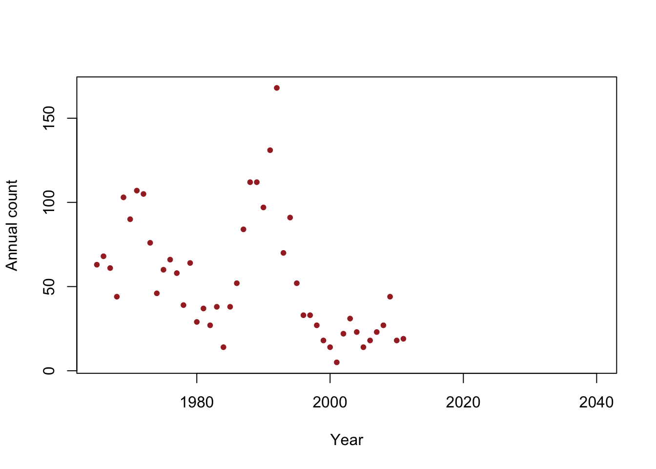
- Is the population size really decreasing?
- Write out the model we should use answer this question
- How can we assess the uncertainty in our estimate of \(\beta_1\)?
- Confidence intervals in R
## (Intercept) year ## 2356.48797 -1.15784## 2.5 % 97.5 % ## (Intercept) 929.80699 3783.1689540 ## year -1.87547 -0.4402103- Note \[\hat{\boldsymbol{\beta}}\sim\text{N}(\boldsymbol{\beta},\sigma^2(\mathbf{X}^{\prime}\mathbf{X})^{-1})\] and let \[\hat{\beta_1}\sim\text{N}(\beta_1,\sigma^{2}_{\beta_1})\] where \(\sigma^{2}_{\beta_1}= \sigma^2\mathbf{c}^{\prime}(\mathbf{X}^{\prime}\mathbf{X})^{-1}\mathbf{c}\) and \(\mathbf{c}\equiv(0,1,0,0,\ldots,0)^{\prime}\). In R we can extract \(\sigma^2(\mathbf{X}^{\prime}\mathbf{X})^{-1}\) using
vcov().
##             (Intercept)         year
## (Intercept) 501753.2825 -252.3792372
## year          -252.3792    0.1269513
Note that
## (Intercept)        year
## 708.3454542   0.3563023
corresponds to the column
Std. Errorfromsummary()## ## Call: ## lm(formula = y ~ year, data = df) ## ## Residuals: ## Min 1Q Median 3Q Max ## -45.333 -20.597 -9.754 14.035 117.929 ## ## Coefficients: ## Estimate Std. Error t value Pr(>|t|) ## (Intercept) 2356.4880 708.3455 3.327 0.00176 ** ## year -1.1578 0.3563 -3.250 0.00219 ** ## --- ## Signif. codes: 0 '***' 0.001 '**' 0.01 '*' 0.05 '.' 0.1 ' ' 1 ## ## Residual standard error: 33.13 on 45 degrees of freedom ## Multiple R-squared: 0.1901, Adjusted R-squared: 0.1721 ## F-statistic: 10.56 on 1 and 45 DF, p-value: 0.00219- When \(\sigma_{\beta_1}\) is known \[\hat{\beta_1}\sim\text{N}(\beta_1,\sigma^{2}_{\beta_1})\] \[\hat{\beta_1} - \beta_1 \sim\text{N}(0,\sigma^{2}_{\beta_1})\] \[\frac{\hat{\beta_1} - \beta_1}{\sigma_{\beta_1}} \sim\text{N}(0,1)\]
- When \(\sigma_{\beta_1}\) is estimated \[\frac{\hat{\beta_1} - \beta_1}{\hat{\sigma}_{\beta_1}} \sim\text{t}(\nu)\] where \(\nu = n - p\)
- Deriving the confidence interval for \(\hat{\beta_1}\) \[\text{P}(a < \frac{\hat{\beta_1} - \beta_1}{\hat{\sigma}_{\beta_1}} < b) = 1-\alpha\] \[\text{P}(a\hat{\sigma}_{\beta_1} < \hat{\beta_1} - \beta_1 < b\hat{\sigma}_{\beta_1}) = 1-\alpha\] \[\text{P}(-\hat{\beta_1} + a\hat{\sigma}_{\beta_1} < - \beta_1 < -\hat{\beta_1} + b\hat{\sigma}_{\beta_1}) = 1-\alpha\] \[\text{P}(\hat{\beta_1} - b\hat{\sigma}_{\beta_1} < \beta_1 < \hat{\beta_1} - a\hat{\sigma}_{\beta_1}) = 1-\alpha\]
- What is \(\text{P}(a < \frac{\hat{\beta_1} - \beta_1}{\hat{\sigma}_{\beta_1}} < b) = 1-\alpha\)? \[\text{P}(a < z < b) = \int_{a}^{b}[z|\nu]dz\]
- “By hand” in R
## [1] -2.014103## [1] 2.014103## year ## -1.87547## year ## -0.4402103## 2.5 % 97.5 % ## -1.8754696 -0.4402103