6 Day 6 (June 8)
6.1 Announcements
Assignment 2 is posted
Recommended reading
- Chapters 2 and 3 (pgs 13 - 46) in Linear Models with R
Questions and comments from journal
- Quick finish to the marathon example…. (link to paper mentioned)
- “If I have a herd of cattle and repeatedly randomly choose 30 cattle, calculating the average weights of each sample. Those samples will eventually form a normal distribution, or a bell-shaped curve.”
- “I understand how the data is collected and it being used to make models. I’m a bit confused on how to transcribe that data and where the equations come from in-order to get from point a to point b. More so in relation to how do you know what to put into Studio or other medias to make them function effectively.”
- “This made me think about how researchers communicate those assumptions and justify their modeling decisions. In my field,biological systems are often complex, so understanding how to combine statistical methods with subject-materer expertisese seems essential for building models that are both accurate and biologically meaningful.”
6.2 Matrix algebra
- Column vectors
- \(\mathbf{y}\equiv(y_{1},y_{2},\ldots,y_{n})^{'}\)
- \(\mathbf{x}\equiv(x_{1},x_{2},\ldots,x_{n})^{'}\)
- \(\boldsymbol{\beta}\equiv(\beta_{1},\beta_{2},\ldots,\beta_{p})^{'}\)
- \(\boldsymbol{1}\equiv(1,1,\ldots,1)^{'}\)
- In R
## [,1] ## [1,] 1 ## [2,] 2 ## [3,] 3 - Matrices
- \(\mathbf{X}\equiv(\mathbf{x}_{1},\mathbf{x}_{2},\ldots,\mathbf{x}_{p})\)
- In R
## [,1] [,2] ## [1,] 1 4 ## [2,] 2 5 ## [3,] 3 6 - Vector multiplication
- \(\mathbf{y}^{'}\mathbf{y}\)
- \(\mathbf{1}^{'}\mathbf{1}\)
- \(\mathbf{1}\mathbf{1}^{'}\)
- In R
## [,1] ## [1,] 14 - Matrix by vector multiplication
- \(\mathbf{X}^{'}\mathbf{y}\)
- In R
## [,1] ## [1,] 14 ## [2,] 32 - Matrix by matrix multiplication
- \(\mathbf{X}^{'}\mathbf{X}\)
- In R
## [,1] [,2] ## [1,] 14 32 ## [2,] 32 77 - Matrix inversion
- \((\mathbf{X}^{'}\mathbf{X})^{-1}\)
- In R
## [,1] [,2] ## [1,] 1.4259259 -0.5925926 ## [2,] -0.5925926 0.2592593 - Determinant of a matrix
- \(|\mathbf{I}|\)
- In R
## [,1] [,2] [,3] ## [1,] 1 0 0 ## [2,] 0 1 0 ## [3,] 0 0 1## [1] 1 - \(|\mathbf{I}|\)
- Quadratic form
- \(\mathbf{y}^{'}\mathbf{S}\mathbf{y}\)
- Derivative of a quadratic form (Note \(\mathbf{S}\) is a symmetric matrix; e.g., \(\mathbf{X}^{'}\mathbf{X}\))
- \(\frac{\partial}{\partial\mathbf{y}}\mathbf{y^{'}\mathbf{S}\mathbf{y}}=2\mathbf{S}\mathbf{y}\)
- Other useful derivatives
- \(\frac{\partial}{\partial\mathbf{y}}\mathbf{\mathbf{x^{'}}\mathbf{y}}=\mathbf{x}\)
- \(\frac{\partial}{\partial\mathbf{y}}\mathbf{\mathbf{X^{'}}\mathbf{y}}=\mathbf{X}\)
6.3 Introduction to linear models
What is a model?
What is a linear model?
Most widely used model in science, engineering, and statistics
Vector form: \(\mathbf{y}=\beta_{0}+\beta_{1}\mathbf{x}_{1}+\beta_{2}\mathbf{x}_{2}+\ldots+\beta_{p}\mathbf{x}_{p}+\boldsymbol{\varepsilon}\)
Matrix form: \(\mathbf{y}=\mathbf{X}\boldsymbol{\beta}+\boldsymbol{\varepsilon}\)
Which part of the model is the mathematical model
Which part of the model makes the linear model a “statistical” model
Visual

Which of the four below are a linear model \[\mathbf{y}=\beta_{0}+\beta_{1}\mathbf{x}_{1}+\beta_{2}\mathbf{x}^{2}_{1}+\boldsymbol{\varepsilon}\] \[\mathbf{y}=\beta_{0}+\beta_{1}\mathbf{x}_{1}+\beta_{2}\text{log(}\mathbf{x}_{1}\text{)}+\boldsymbol{\varepsilon}\] \[\mathbf{y}=\beta_{0}+\beta_{1}e^{\beta_{2}\mathbf{x}_{1}}+\boldsymbol{\varepsilon}\] \[\mathbf{y}=\beta_{0}+\beta_{1}\mathbf{x}_{1}+\text{log(}\beta_{2}\text{)}\mathbf{x}_{1}+\boldsymbol{\varepsilon}\]
Why study the linear model?
- Building block for more complex models (e.g., GLMs, mixed models, machine learning, etc)
- We know the most about it
6.4 Estimation
- Three options to estimate \(\boldsymbol{\beta}\)
- Minimize a loss function
- Maximize a likelihood function
- Find the posterior distribution
- Each option requires different assumptions
6.5 Loss function approach
- Define a measure of discrepancy between the data and the mathematical model
- Find the values of \(\boldsymbol{\beta}\) that make \(\mathbf{X}\boldsymbol{\beta}\) “closest” to \(\mathbf{y}\)
- Visual
- Classic example \[\underset{\boldsymbol{\beta}}{\operatorname{argmin}}\sum_{i=1}^{n}(y_i-\mathbf{x}_{i}^{\prime}\boldsymbol{\beta})^2\] or in matrix form \[\underset{\boldsymbol{\beta}}{\operatorname{argmin}}(\mathbf{y} - \mathbf{X}\boldsymbol{\beta})^{\prime}(\mathbf{y} - \mathbf{X}\boldsymbol{\beta})\] which results in \[\hat{\boldsymbol{\beta}}=(\mathbf{X}^{\prime}\mathbf{X})^{-1}\mathbf{X}^{\prime}\mathbf{y}\]
- Three ways to do it in program R
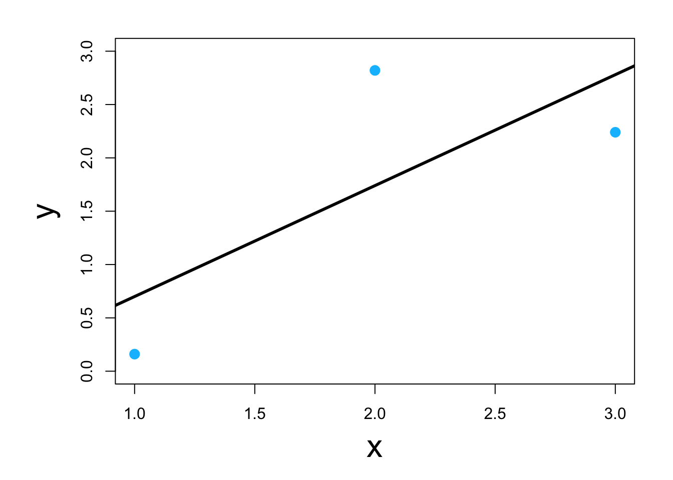
- Using scalar calculus and algebra (kind of)
y <- c(0.16,2.82,2.24)
x <- c(1,2,3)

y.bar <- mean(y)
x.bar <- mean(x)

# Estimate the slope parameter
beta1.hat <- sum((x-x.bar)*(y-y.bar))/sum((x-x.bar)^2)
beta1.hat
## [1] 1.04# Estimate the intercept parameter beta0.hat <- y.bar - sum((x-x.bar)*(y-y.bar))/sum((x-x.bar)^2)*x.bar beta0.hat## [1] -0.34