3 Day 3 (June 3)
3.1 Announcements
Friday donuts and extra credit!
Assignment 1 is due on Friday.
- Upload to Canvas
- Assignment should only take 15-30 min if everything works
- Do not spend more than 1 hour
- After 1 hour of trying please visit me during office hours
- Do not wait until Thursday to do the assignment
Recommended reading
- Chapters 1 and 2 (pgs 1 - 27) in Linear Models with R
Questions and comments from journal
- “Something that I found interesting and learned in the last 24 hours in this course is how statistical models can be used to answer questions even when we do not have all the information.”
- “The difference between point prediction and distributional prediction needs more clarification.” (see satirical articles here)
- “The transition from personal information to a generalized statistical model was not clear to me.”
- “I would like to understand how to know which model to run and why. Does it depend on the data collected and the question being asked or just one of the two?”
- “Can you run different types of models with the same data set and get similar results or would the results be all wonky with one type of model and accurate with another and that is where the beauty of understanding statistics comes in?”
3.2 Intro to statistical modelling: retirment example
Goal of the next few days is to get excited about statistical modeling
Discussion question: How much data do you need to do statistics?
A difficult question
- “How much money will I have for retirement?”
- “Am I ruining my life now by over saving for retirement?”
What is data?
- Something in the real world that you can, in some way, observe and measure with or without error
What is a statistic?
- A function of the data
What is a model?
- Mathematical models
- Statistical models
Back to the difficult question
- How much money will I have for retirement?
- Point prediction vs. distributional prediction
- What data/information do I have?
- What data do I need?
- How can I answer this question using a statistical model?
- How much money will I have for retirement?
Example: my retirement
- Personal information
- Obviously this isn’t my actual information, but it isn’t too far off!
- Since I am a millennial I don’t think social security will be around when I retire (i.e., assume social security contributes $0 to my retirement)
- As of 1/1/26 I have $600,000 in a 401k style retirement account
- All of money is invested into an S&P 500 index fund (VOO to be exact)
- I am 40 as of 1/1/26
- I want to know how much pre-tax money I will have at a given retirement age (e.g., 65, 70, etc)
- Example using a mathematical model
- Whiteboard demonstration
- What are the model assumptions?
- In program R
- Personal information
# The value of my 401k retirement account as of 1/1/26
y_2026 <- 600000


# How much money will I add to my 401k each year
q <- 28000


# Rate of return for S&P 500 index fund
r <- 0.08


# How much $ will I have in 2027
y_2027 <- y_2026*(1+r)+q
y_2027
## [1] 676000## [1] 758080## [1] 846726.4# Using a for loop to calculate how much $ will I have
year <- seq(2026,2026+30,by=1)
y <- matrix(,length(year),1)
rownames(y) <- year
y[1,1] <- 600000
for(t in 1:30){
y[t+1,1] <- y[t,1]*(1+r)+q
}
plot(year,y/10^6,typ="b",pch=20,col="deepskyblue",xlab="Year",ylab="Pretax retirement amount ($ millions)")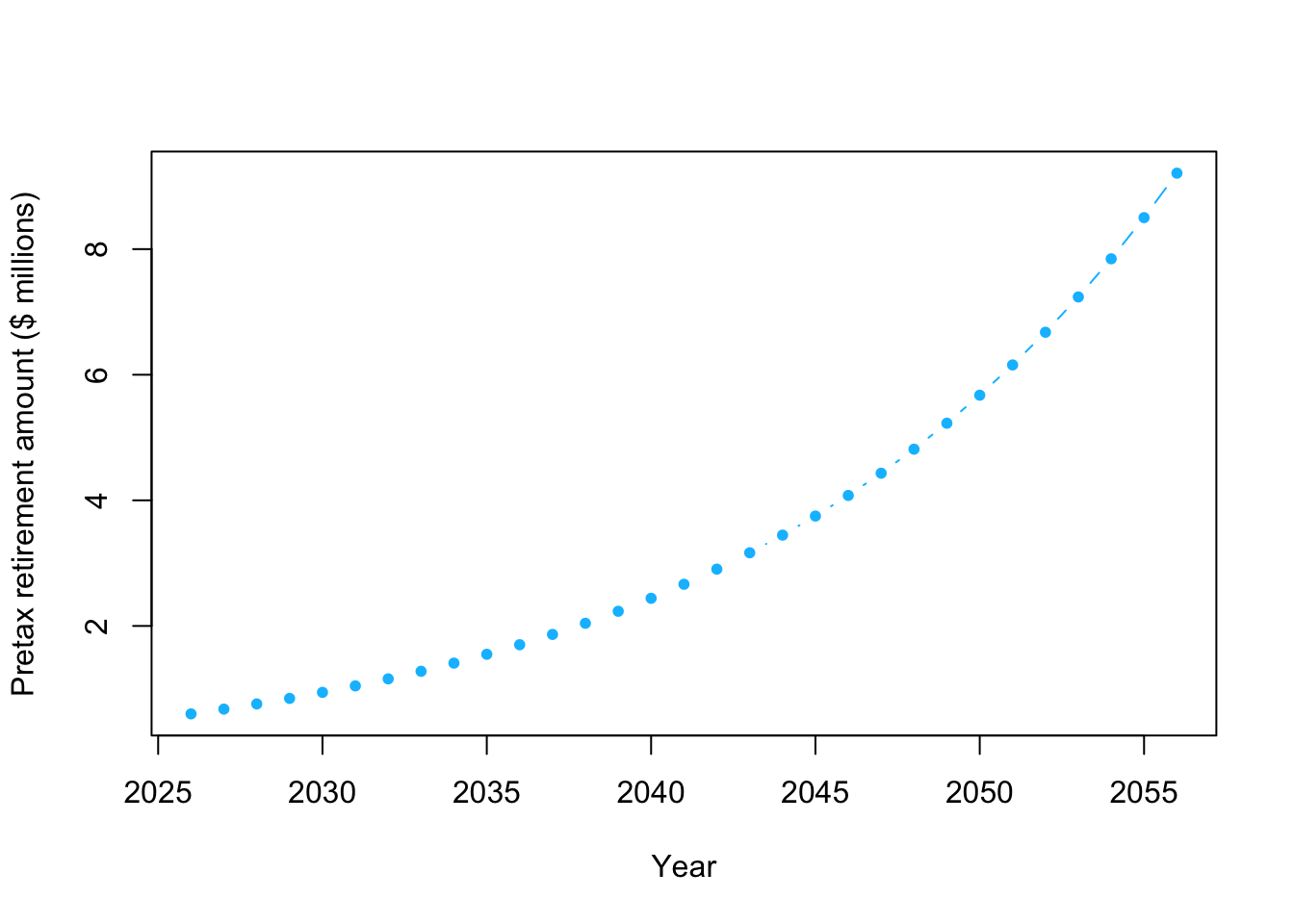
# How much $ will I have when I am 60?
# Note that units are millions of $
retirement.year <- 2026+20
y[which(year==retirement.year)]/10^6
## [1] 4.077909- Example using a Bayesian statistical model
- S&P 500 return since inception in 1957
# Download S&P 500 returns
url <- "https://www.dropbox.com/scl/fi/cgnf2tt64qi4uososhdnf/chart_20260529T205422.csv?rlkey=nampviv31g3p2k39q91km3cf4&dl=1"
df.sp500 <- read.csv(url)

head(df.sp500)
## Date return
## 1 12/31/57 -0.1431
## 2 12/31/58 0.3806
## 3 12/31/59 0.0848
## 4 12/31/60 -0.0297
## 5 12/31/61 0.2313
## 6 12/31/62 -0.1181## Date return
## 64 12/31/20 0.1626
## 65 12/31/21 0.2689
## 66 12/31/22 -0.1944
## 67 12/31/23 0.2423
## 68 12/31/24 0.2331
## 69 12/31/25 0.1639## [1] 0.08838116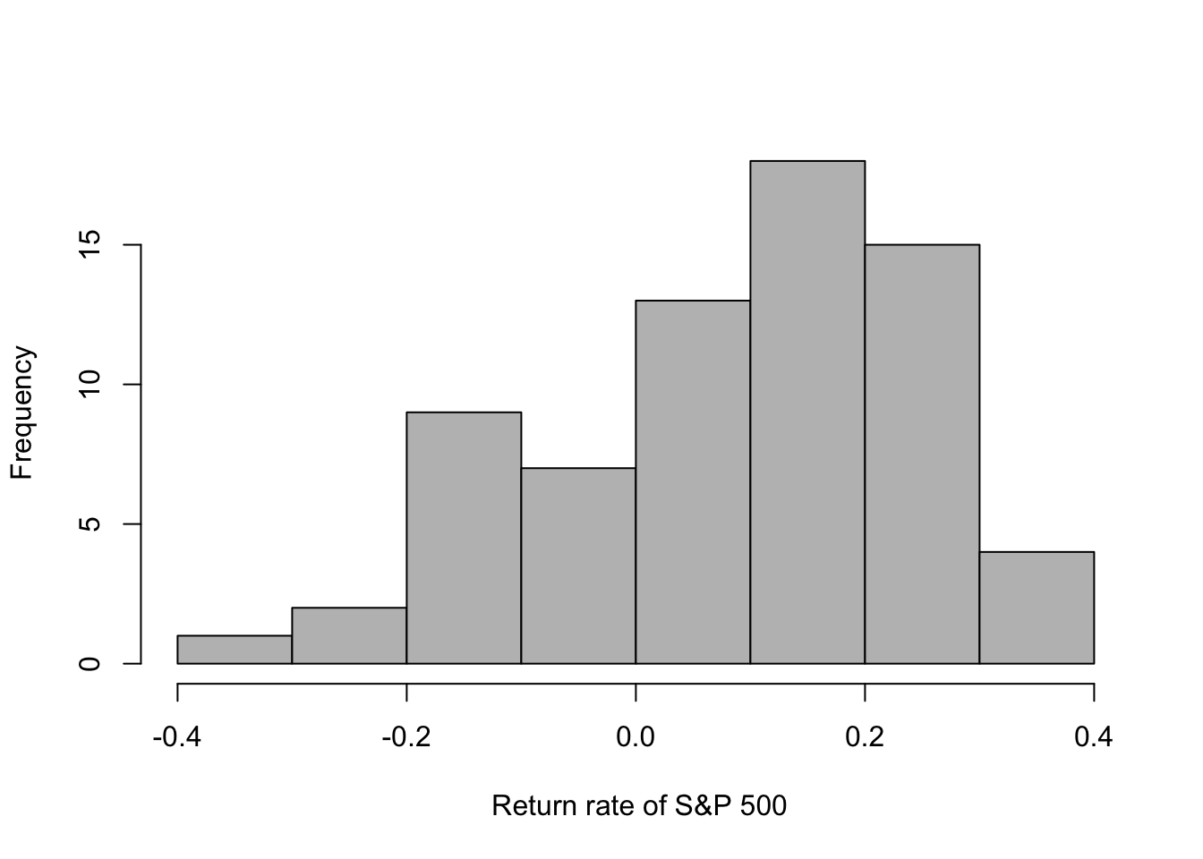 - Example using the prior predictive distribution
# Download S&P 500 returns
url <- "https://www.dropbox.com/scl/fi/cgnf2tt64qi4uososhdnf/chart_20260529T205422.csv?rlkey=nampviv31g3p2k39q91km3cf4&dl=1"
df.sp500 <- read.csv(url)

# The value of my 401k retirement account as of 1/1/26
y_2026 <- 600000

# How much money will I add to my 401k each year
q <- 28000


# Using a for loop to calculate how much $ will I have
year <- seq(2026,2026+30,by=1)
Y <- matrix(,length(year),1000)
rownames(Y) <- year
Y[1,] <- y_2026

set.seed(3410)
for(m in 1:1000){
for(t in 1:30){
  r <- sample(df.sp500$return,1)
  Y[t+1,m] <- Y[t,m]*(1+r)+q
              }
                }


# Prior predictive distribution for a given year
retirement.year <- 2026+20
hist(Y[which(year==retirement.year),]/10^6,col="grey",freq=FALSE,xlab="Pretax retirement amount ($ millions)",main="")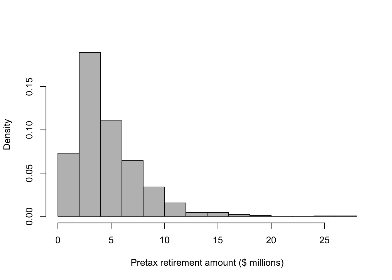
## [1] 4.695358## [1] 27.0164## [1] 0.5515685## 2.5% 97.5%
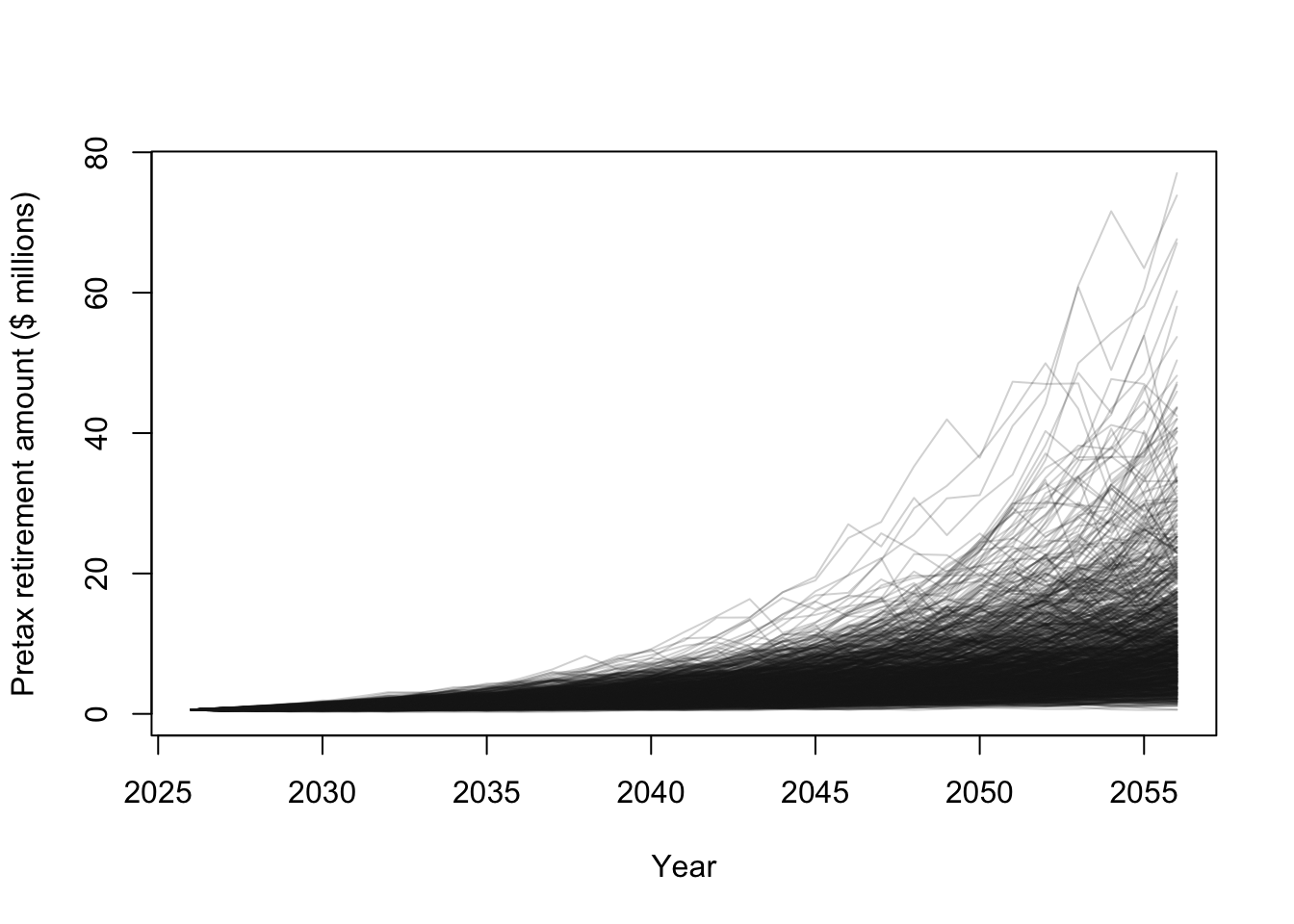
## 1.213856 12.129545# Plot some financial trajectories (i.e., random draws from the prior predictive distribution)
plot(year,Y[,1]/10^6,typ="l",lwd=1,ylim=c(0,max(Y/10^6)),col=rgb(0.1,0.1,0.1,.05),xlab="Year",ylab="Pretax retirement amount ($ millions)")
for(i in 1:1000){
points(year,Y[,i]/10^6,typ="l",lwd=1,col=rgb(0.1,0.1,0.1,.2))
}
# Plot of prior predictive distribution for all years
E.Y <- apply(Y/10^6,1,mean)
u.CI <- apply(Y/10^6,1,quantile,prob=0.975)
l.CI <- apply(Y/10^6,1,quantile,prob=0.025)
max.Y <- apply(Y/10^6,1,max)
min.Y <- apply(Y/10^6,1,min)

plot(year,E.Y,typ="l",lwd=3,ylim=c(0,max(max.Y)),xlab="Year",ylab="Pretax retirement amount ($ millions)")
points(year,max.Y,typ="l",lwd=3,col="red")
points(year,min.Y,typ="l",lwd=3,col="red")
polygon(c(year,rev(year)),c(u.CI,rev(l.CI)),
        col=rgb(0.5,0.5,0.5,0.5),border=rgb(0.5,0.5,0.5,0.5))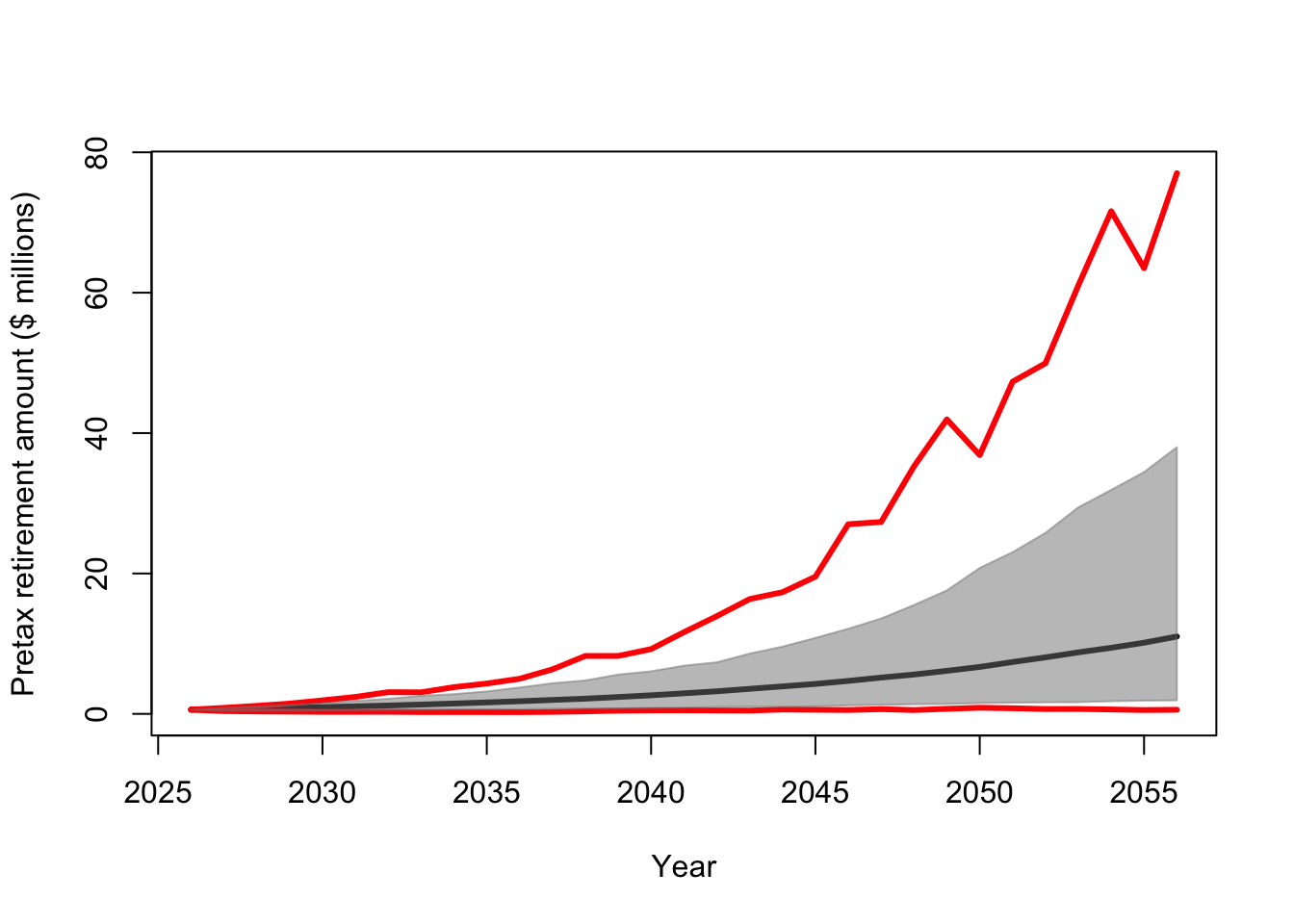
- Further reading/learning
3.3 Intro to statistical modelling: human movement
- The goal of this activity is to show you how cool spatio-temporal statistics is!
- Human movement modeling with the linear regression model and other fancy tools!
- Trajectories are a time series of the spatial location of an object (or animal).
- We can usually pick the object and the time that we obtain its spatial location (i.e., time is fixed)
- The location is a random variable in most cases, but time can also be a random variable.
- In-class marathon example (Download R script here)
- Further reading/learning
- Hooten, M.B, D.S. Johnson, D.S., B.T. McClintock, J.M. Morales (2017) Animal Movement: Statistical Models for Telemetry Data. CRC press