8 Day 8 (June 10)
8.1 Announcements
Assignment 2 is posted
Recommended reading
- Chapters 2 and 3 (pgs 13 - 46) in Linear Models with R
Questions and comments from journal
“I am struggling to understand how the polynomial regression can also be considered as a linear regression.”
“As we’ve discussed, statistics is an art, but what is we don’t know the mathematical shape or slope that an explanatory variable should or will take on.”(link to ASFV paper)
“On the other hand, something that was not clear to me in class was how we can visualize a model with more than two variables”
8.2 Introduction to linear models
What is a model?
What is a linear model?
Most widely used model in science, engineering, and statistics
Vector form: \(\mathbf{y}=\beta_{0}+\beta_{1}\mathbf{x}_{1}+\beta_{2}\mathbf{x}_{2}+\ldots+\beta_{p}\mathbf{x}_{p}+\boldsymbol{\varepsilon}\)
Matrix form: \(\mathbf{y}=\mathbf{X}\boldsymbol{\beta}+\boldsymbol{\varepsilon}\)
Which part of the model is the mathematical model
Which part of the model makes the linear model a “statistical” model
Visual
Which of the four below are a linear model \[\mathbf{y}=\beta_{0}+\beta_{1}\mathbf{x}_{1}+\beta_{2}\mathbf{x}^{2}_{1}+\boldsymbol{\varepsilon}\] \[\mathbf{y}=\beta_{0}+\beta_{1}\mathbf{x}_{1}+\beta_{2}\text{log(}\mathbf{x}_{1}\text{)}+\boldsymbol{\varepsilon}\] \[\mathbf{y}=\beta_{0}+\beta_{1}e^{\beta_{2}\mathbf{x}_{1}}+\boldsymbol{\varepsilon}\] \[\mathbf{y}=\beta_{0}+\beta_{1}\mathbf{x}_{1}+\text{log(}\beta_{2}\text{)}\mathbf{x}_{1}+\boldsymbol{\varepsilon}\]
Why study the linear model?
- Building block for more complex models (e.g., GLMs, mixed models, machine learning, etc)
- We know the most about it
8.3 Estimation
- Three options to estimate \(\boldsymbol{\beta}\)
- Minimize a loss function
- Maximize a likelihood function
- Find the posterior distribution
- Each option requires different assumptions
8.4 Loss function approach
- Define a measure of discrepancy between the data and the mathematical model
- Find the values of \(\boldsymbol{\beta}\) that make \(\mathbf{X}\boldsymbol{\beta}\) “closest” to \(\mathbf{y}\)
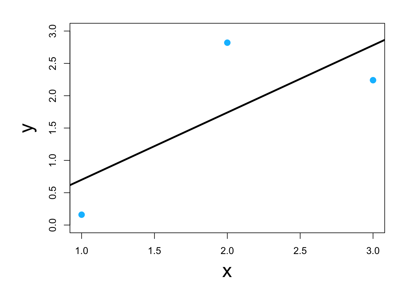
- Visual
- Classic example \[\underset{\boldsymbol{\beta}}{\operatorname{argmin}}\sum_{i=1}^{n}(y_i-\mathbf{x}_{i}^{\prime}\boldsymbol{\beta})^2\] or in matrix form \[\underset{\boldsymbol{\beta}}{\operatorname{argmin}}(\mathbf{y} - \mathbf{X}\boldsymbol{\beta})^{\prime}(\mathbf{y} - \mathbf{X}\boldsymbol{\beta})\] which results in \[\hat{\boldsymbol{\beta}}=(\mathbf{X}^{\prime}\mathbf{X})^{-1}\mathbf{X}^{\prime}\mathbf{y}\]
- Three ways to do it in program R

- Using scalar calculus and algebra (kind of)
y <- c(0.16,2.82,2.24)
x <- c(1,2,3)

y.bar <- mean(y)
x.bar <- mean(x)

# Estimate the slope parameter
beta1.hat <- sum((x-x.bar)*(y-y.bar))/sum((x-x.bar)^2)
beta1.hat
## [1] 1.04# Estimate the intercept parameter beta0.hat <- y.bar - sum((x-x.bar)*(y-y.bar))/sum((x-x.bar)^2)*x.bar beta0.hat## [1] -0.34 - Live example