13 Day 13 (June 17)
13.1 Announcements
Any questions about assignment 3?
Recommended reading
- Chapters 4 (pgs 42-58) in Linear Models with R
Questions and comments from journal
- Probability distributions commonly used in statistics
- “Something that I learned from class is that even if we don’t have a large dataset, the results can still be reliable.”
- “Something I’m still trying to understand is whether we can create models for everything, or if there are situations where models do not work at all. I also know that there are distributions other than the normal distribution that can be used in modeling. However, can we always use the normality assumption, or are there scenarios in which we definitely cannot assume a normal distribution.”
- “For clarification, we are learning the statistics to do before linear regression or different types of ways to do linear regression? Do all models with assumptions come with them built in and we add on or is maximum likelihood estimation one of few models with set assumptions?”
13.2 Confidence intervals for paramters
Example
y <- c(63, 68, 61, 44, 103, 90, 107, 105, 76, 46, 60, 66, 58, 39, 64, 29, 37,
27, 38, 14, 38, 52, 84, 112, 112, 97, 131, 168, 70, 91, 52, 33, 33, 27,
18, 14, 5, 22, 31, 23, 14, 18, 23, 27, 44, 18, 19)
year <- 1965:2011
df <- data.frame(y = y, year = year)
plot(x = df$year, y = df$y, xlab = "Year", ylab = "Annual count", main = "",
col = "brown", pch = 20, xlim = c(1965, 2040))
- Is the population size really decreasing?
- Write out the model we should use answer this question
- How can we assess the uncertainty in our estimate of \(\beta_1\)?
- Confidence intervals in R
## (Intercept) year ## 2356.48797 -1.15784## 2.5 % 97.5 % ## (Intercept) 929.80699 3783.1689540 ## year -1.87547 -0.4402103- Note \[\hat{\boldsymbol{\beta}}\sim\text{N}(\boldsymbol{\beta},\sigma^2(\mathbf{X}^{\prime}\mathbf{X})^{-1})\] and let \[\hat{\beta_1}\sim\text{N}(\beta_1,\sigma^{2}_{\beta_1})\] where \(\sigma^{2}_{\beta_1}= \sigma^2\mathbf{c}^{\prime}(\mathbf{X}^{\prime}\mathbf{X})^{-1}\mathbf{c}\) and \(\mathbf{c}\equiv(0,1,0,0,\ldots,0)^{\prime}\). In R we can extract \(\sigma^2(\mathbf{X}^{\prime}\mathbf{X})^{-1}\) using
vcov().
##             (Intercept)         year
## (Intercept) 501753.2825 -252.3792372
## year          -252.3792    0.1269513
Note that
## (Intercept)        year
## 708.3454542   0.3563023
corresponds to the column
Std. Errorfromsummary()## ## Call: ## lm(formula = y ~ year, data = df) ## ## Residuals: ## Min 1Q Median 3Q Max ## -45.333 -20.597 -9.754 14.035 117.929 ## ## Coefficients: ## Estimate Std. Error t value Pr(>|t|) ## (Intercept) 2356.4880 708.3455 3.327 0.00176 ** ## year -1.1578 0.3563 -3.250 0.00219 ** ## --- ## Signif. codes: 0 '***' 0.001 '**' 0.01 '*' 0.05 '.' 0.1 ' ' 1 ## ## Residual standard error: 33.13 on 45 degrees of freedom ## Multiple R-squared: 0.1901, Adjusted R-squared: 0.1721 ## F-statistic: 10.56 on 1 and 45 DF, p-value: 0.00219- When \(\sigma_{\beta_1}\) is known \[\hat{\beta_1}\sim\text{N}(\beta_1,\sigma^{2}_{\beta_1})\] \[\hat{\beta_1} - \beta_1 \sim\text{N}(0,\sigma^{2}_{\beta_1})\] \[\frac{\hat{\beta_1} - \beta_1}{\sigma_{\beta_1}} \sim\text{N}(0,1)\]
- When \(\sigma_{\beta_1}\) is estimated \[\frac{\hat{\beta_1} - \beta_1}{\hat{\sigma}_{\beta_1}} \sim\text{t}(\nu)\] where \(\nu = n - p\)
- Deriving the confidence interval for \(\hat{\beta_1}\) \[\text{P}(a < \frac{\hat{\beta_1} - \beta_1}{\hat{\sigma}_{\beta_1}} < b) = 1-\alpha\] \[\text{P}(a\hat{\sigma}_{\beta_1} < \hat{\beta_1} - \beta_1 < b\hat{\sigma}_{\beta_1}) = 1-\alpha\] \[\text{P}(-\hat{\beta_1} + a\hat{\sigma}_{\beta_1} < - \beta_1 < -\hat{\beta_1} + b\hat{\sigma}_{\beta_1}) = 1-\alpha\] \[\text{P}(\hat{\beta_1} - b\hat{\sigma}_{\beta_1} < \beta_1 < \hat{\beta_1} - a\hat{\sigma}_{\beta_1}) = 1-\alpha\]
- What is \(\text{P}(a < \frac{\hat{\beta_1} - \beta_1}{\hat{\sigma}_{\beta_1}} < b) = 1-\alpha\)? \[\text{P}(a < z < b) = \int_{a}^{b}[z|\nu]dz\]
- “By hand” in R
## [1] -2.014103## [1] 2.014103## year ## -1.87547## year ## -0.4402103## 2.5 % 97.5 % ## -1.8754696 -0.4402103
13.3 Confidence intervals for derived quantities
Demonstration of how not to do it.
y <- c(63, 68, 61, 44, 103, 90, 107, 105, 76, 46, 60, 66, 58, 39, 64, 29, 37,
27, 38, 14, 38, 52, 84, 112, 112, 97, 131, 168, 70, 91, 52, 33, 33, 27,
18, 14, 5, 22, 31, 23, 14, 18, 23, 27, 44, 18, 19)
year <- 1965:2011
df <- data.frame(y = y, year = year)
plot(x = df$year, y = df$y, xlab = "Year", ylab = "Annual count", main = "",
col = "brown", pch = 20, xlim = c(1965, 2040))
## (Intercept) year ## 2356.48797 -1.15784## 2.5 % 97.5 % ## (Intercept) 929.80699 3783.1689540 ## year -1.87547 -0.4402103# This is ok! beta0.hat <- as.numeric(coef(m1)[1]) beta1.hat <- as.numeric(coef(m1)[2]) extinct.date.hat <- -beta0.hat/beta1.hat extinct.date.hat## [1] 2035.245# This is not ok! beta0.hat.li <- confint(m1)[1,1] beta1.hat.li <- confint(m1)[2,1] extinct.date.li <- -beta0.hat.li/beta1.hat.li extinct.date.li## [1] 495.7729beta0.hat.ui <- confint(m1)[1,2] beta1.hat.ui <- confint(m1)[2,2] extinct.date.ui <- -beta0.hat.ui/beta1.hat.ui extinct.date.ui## [1] 8594.004The delta method
- See (ver2012invented?) and (powell2007approximating?) for more info
library(msm)

y <- c(63, 68, 61, 44, 103, 90, 107, 105, 76, 46, 60, 66, 58, 39, 64, 29, 37, 27,
    38, 14, 38, 52, 84, 112, 112, 97, 131, 168, 70, 91, 52, 33, 33, 27, 18, 14, 5,
    22, 31, 23, 14, 18, 23, 27, 44, 18, 19)
year <- 1965:2011
df <- data.frame(y = y, year = year)
plot(x = df$year, y = df$y, xlab = "Year", ylab = "Annual count", main = "", col = "brown",
    pch = 20, xlim = c(1965, 2040))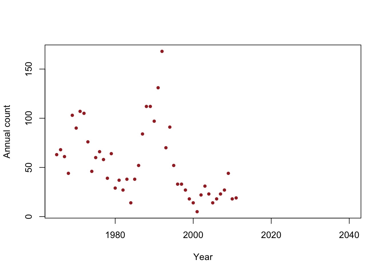
## (Intercept) year ## 2356.48797 -1.15784## 2.5 % 97.5 % ## (Intercept) 929.80699 3783.1689540 ## year -1.87547 -0.4402103beta0.hat <- as.numeric(coef(m1)[1]) beta1.hat <- as.numeric(coef(m1)[2]) extinct.date.hat <- -beta0.hat/beta1.hat extinct.date.hat## [1] 2035.245extinct.date.se <- deltamethod(~-x1/x2, mean = coef(m1), cov = vcov(m1)) extinct.date.ci <- c(extinct.date.hat - 1.96 * extinct.date.se, extinct.date.hat + 1.96 * extinct.date.se) extinct.date.ci## [1] 2005.598 2064.892