9 Day 9 (June 11)
9.1 Announcements
Assignment 1 is graded
- If you do not like your grade, please email me (thefley@ksu.edu) a revised assignment by next Monday.
Cool youtube video about using statistics to predict deer health (link)
Recommended reading
- Chapters 2 and 3 (pgs 13 - 46) in Linear Models with R
Questions and comments from journal
- “Has there been moments in your career where people that aren’t in your field have taught you something new?”
- “Something that I would like to understand better is for the loss function approach: how is it decided which best fit line is used or which equation. I understand how they are measured but is it just a different way to see the information? When and how do you decide what to use? Do you just go with what is most widely accepted or popular?”
- “The thing I’m a bit confused about is absolute loss and what is being lost if anything? I know in statistics there is a lot of terminology used that have different meanings sometimes different from what it can be defined as. What exactly does the loss have to do with less squares and that determining the distance alongside that?”
- “One thing I am still trying to understand is why minimizing the squared error yields the specific formulas for the slope and intercept.”
- “I am still struggling to understand why the values for least squares and absolute loss are not consistent.”
- “I am able to find sire and dam LTE, color, year foaled, and sex easily online but worry there won’t be enough correlation to the horse’s LTE to find anything interesting.”
9.2 Estimation
- Three options to estimate \(\boldsymbol{\beta}\)
- Minimize a loss function
- Maximize a likelihood function
- Find the posterior distribution
- Each option requires different assumptions
9.3 Loss function approach
- Define a measure of discrepancy between the data and the mathematical model
- Find the values of \(\boldsymbol{\beta}\) that make \(\mathbf{X}\boldsymbol{\beta}\) “closest” to \(\mathbf{y}\)
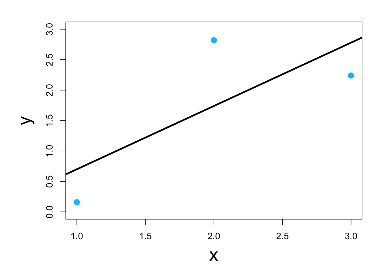
- Visual
- Classic example \[\underset{\boldsymbol{\beta}}{\operatorname{argmin}}\sum_{i=1}^{n}(y_i-\mathbf{x}_{i}^{\prime}\boldsymbol{\beta})^2\] or in matrix form \[\underset{\boldsymbol{\beta}}{\operatorname{argmin}}(\mathbf{y} - \mathbf{X}\boldsymbol{\beta})^{\prime}(\mathbf{y} - \mathbf{X}\boldsymbol{\beta})\] which results in \[\hat{\boldsymbol{\beta}}=(\mathbf{X}^{\prime}\mathbf{X})^{-1}\mathbf{X}^{\prime}\mathbf{y}\]
- Three ways to do it in program R
- Using scalar calculus and algebra (kind of)
y <- c(0.16,2.82,2.24)
x <- c(1,2,3)

y.bar <- mean(y)
x.bar <- mean(x)

# Estimate the slope parameter
beta1.hat <- sum((x-x.bar)*(y-y.bar))/sum((x-x.bar)^2)
beta1.hat
## [1] 1.04# Estimate the intercept parameter beta0.hat <- y.bar - sum((x-x.bar)*(y-y.bar))/sum((x-x.bar)^2)*x.bar beta0.hat## [1] -0.34- Using matrix calculus and algebra
y <- c(0.16,2.82,2.24)
X <- matrix(c(1,1,1,1,2,3),nrow=3,ncol=2,byrow=FALSE)
solve(t(X)%*%X)%*%t(X)%*%y
## [,1] ## [1,] -0.34 ## [2,] 1.04- Using modern (circa 1970’s) optimization techniques
y <- c(0.16,2.82,2.24)
x <- c(1,2,3)

optim(par=c(0,0),method = c("Nelder-Mead"),fn=function(beta){sum((y-(beta[1]+beta[2]*x))^2)})
## $par ## [1] -0.3399977 1.0399687 ## ## $value ## [1] 1.7496 ## ## $counts ## function gradient ## 61 NA ## ## $convergence ## [1] 0 ## ## $message ## NULL- Using modern and user friendly statistical computing software
## ## Call: ## lm(formula = y ~ x, data = df) ## ## Coefficients: ## (Intercept) x ## -0.34 1.04 - Live example
9.4 Maximum Likelihood Estimation
- Maximum likelihood estimation for the linear model
- Assume that \(\mathbf{y}\sim \text{N}(\mathbf{X}\boldsymbol{\beta},\sigma^2\mathbf{I})\)
- Write out the likelihood function \[\mathcal{L}(\boldsymbol{\beta},\sigma^2)=\prod_{i=1}^n\frac{1}{\sqrt{2\pi\sigma^2}}\textit{e}^{-\frac{1}{2\sigma^2}(y_{i} - \mathbf{x}_{i}^{\prime}\boldsymbol{\beta})^2}.\]
- Maximize the likelihood function
- First take the natural log of \(\mathcal{L}(\boldsymbol{\beta},\sigma^2)\), which gives \[\mathcal{l}(\boldsymbol{\beta},\sigma^2)=-\frac{n}{2}\text{ log}(2\pi\sigma^2) - \frac{1}{2\sigma^2}\sum_{i=1}^{n}(y_{i} - \mathbf{x}_{i}^{\prime}\boldsymbol{\beta})^2.\]
- Recall that \(\sum_{i=1}^{n}(y_{i} - \mathbf{x}_{i}^{\prime}\boldsymbol{\beta})^2 = (\mathbf{y} - \mathbf{X}\boldsymbol{\beta})^{\prime}(\mathbf{y} - \mathbf{X}\boldsymbol{\beta})\)
- Maximize the log-likelihood function \[\underset{\boldsymbol{\beta}, \sigma^2}{\operatorname{argmax}} -\frac{n}{2}\text{ log}(2\pi\sigma^2) - \frac{1}{2\sigma^2}(\mathbf{y} - \mathbf{X}\boldsymbol{\beta})^{\prime}(\mathbf{y} - \mathbf{X}\boldsymbol{\beta})\]
- Visual for data \(\mathbf{y}=(0.16,2.82,2.24)'\) and \(\mathbf{x}=(1,2,3)'\)
- Three ways to do it in program R
- Using matrix calculus and algebra
# Data
y <- c(0.16,2.82,2.24)
X <- matrix(c(1,1,1,1,2,3),nrow=3,ncol=2,byrow=FALSE)
n <- length(y)

# Maximum likelihood estimation using closed from estimators
beta <- solve(t(X)%*%X)%*%t(X)%*%y
sigma2 <- (1/n)*t(y-X%*%beta)%*%(y-X%*%beta)

beta
## [,1] ## [1,] -0.34 ## [2,] 1.04## [,1] ## [1,] 0.5832- Using modern (circa 1970’s) optimization techniques
# Maximum likelihood estimation estimation using the Nelder-Mead algorithm
y <- c(0.16,2.82,2.24)
X <- matrix(c(1,1,1,1,2,3),nrow=3,ncol=2,byrow=FALSE)

negloglik <- function(par){
beta <- par[1:2]
sigma2 <- par[3]
-sum(dnorm(y,X%*%beta,sqrt(sigma2),log=TRUE))
}
optim(par=c(0,0,1),fn=negloglik,method = "Nelder-Mead")
## $par ## [1] -0.3397162 1.0398552 0.5831210 ## ## $value ## [1] 3.447978 ## ## $counts ## function gradient ## 150 NA ## ## $convergence ## [1] 0 ## ## $message ## NULL- Using modern and user friendly statistical computing software
# Maximum likelihood estimation using lm function
# Note: estimate of sigma2 is not the MLE!
df <- data.frame(y = c(0.16,2.82,2.24),x = c(1,2,3))
m1 <- lm(y~x,data=df)

coef(m1)
## (Intercept) x ## -0.34 1.04## [1] 1.7496## ## Call: ## lm(formula = y ~ x, data = df) ## ## Residuals: ## 1 2 3 ## -0.54 1.08 -0.54 ## ## Coefficients: ## Estimate Std. Error t value Pr(>|t|) ## (Intercept) -0.3400 2.0205 -0.168 0.894 ## x 1.0400 0.9353 1.112 0.466 ## ## Residual standard error: 1.323 on 1 degrees of freedom ## Multiple R-squared: 0.5529, Adjusted R-squared: 0.1057 ## F-statistic: 1.236 on 1 and 1 DF, p-value: 0.4663